05b Observation with Sol'Ex - Part 2 (SolEx)

In addition to Sol'Ex, you will need a filter holder, which is easy to 3D print and install, and inexpensive 3D cinema glasses:

 

Above, the filter holder that you attach to the Sol'Ex entrance, and a set of two polarizing filter holders. Below, a pair of 3D viewing glasses from which you can obtain the polarizing filters that respond to circular polarization.

To download the STL files for printing the filter holder elements, click here.

click here

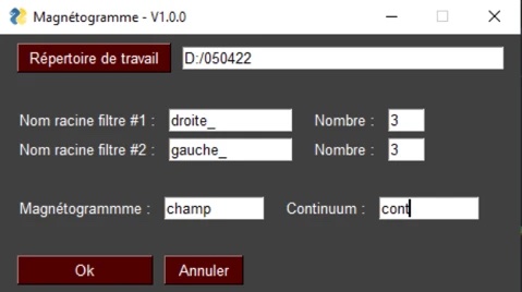
If you watch the above-mentioned video on observing the sun's magnetic field, you will notice that data processing is easier if you use INTI version 3.2.0 and higher (download from the usual website) and a small add-on program called "magnet.exe."

The latter very quickly performs the centering and image stitching operations necessary for synthesizing the magnetogram. To download the MAGNET application, click here, unzip the ZIP file, and launch the executable file as usual in Windows (you can create a shortcut on your desktop). An English version is also available here.
 

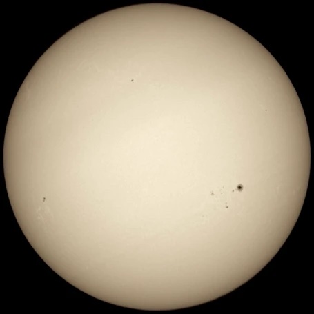
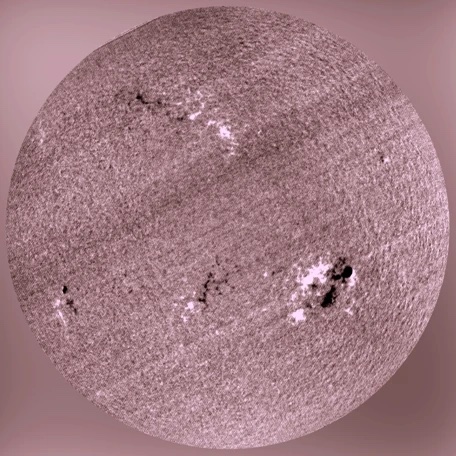
On the left is the image of the Sun on April 5, 2022, taken in white light with a Sol'Ex in conjunction with a Sky-Watcher 72ED refractor and a HOYA ND16 filter as input (for polarimetric observations, it is not possible to use a Herschel helioscope configuration, as this creates its own polarization, which obscures the desired information). On the right is the Sol'Ex magnetogram for the same date. It can be seen that the active centers are bipolar elements and that the sign of the magnetic field is reversed between the Northern and Southern Hemispheres (north is at the top in these images).

Part 16: The "Cinematic" Observation

Let's not forget that the Sun is a dynamic celestial body with changes that can occur very quickly.

Part 17: How to find your way around the Sun's spectrum?

While a novice spectrographer can successfully use Sol Ex, it must be admitted that first encountering a star's spectrum can be confusing if you've never encountered such a situation before. To help you navigate and understand what a stellar spectrum is—that "barcode" that represents the star's physical signature—I recommend downloading an atlas of the solar spectrum by Olivier Garde by clicking on the image below. In a single image and in visual colors, you'll get a global view of the solar spectrum, with the additional identification of the chemical element responsible for this or that line. This magnificent work by Olivier was carried out using an ESP-scale spectrograph (Shelyak Instruments) with very high resolution (R=30,000, which means that the fineness of the details in the wavelength is equal to the wavelength divided by 30,000).

A very useful exercise is to compare Olivier's spectral map with the actual data from Sol'Ex. You can explore the spectral range by moving the circular lever that drives the grating in one direction or the other (Note: You may need to adjust the camera settings to focus on the observed spectral range, as the lenses used in Sol'Ex have residual chromatism). One minor difficulty is that the spectrum reproduced by the camera is in grayscale, while Olivier's spectrum is in color. The exercise consists of identifying the barcode motifs between the two at the end of the code. You'll be surprised how quickly you'll be able to do this, as if reading a road map. The Sun's spectrum will become your territory!

See also the video guide in Part 14 of the "Setup" section of this website or the excerpts from the Sol'Ex spectra below.

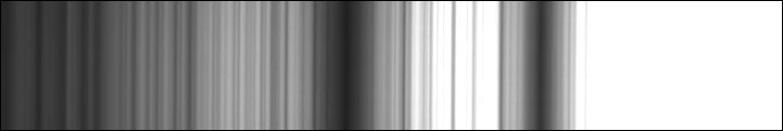
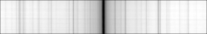
We'll start with the H and K lines of uniquely ionized calcium (Ca II). They are located at the boundary between blue and ultraviolet, at a wavelength of 3950 angstroms. The K line is on the left in this image, the H line on the right. These are very wide notches in the color "continuum" of the spectrum (this is the rule; in graphic representations with a horizontal spectrum, the lengths must always increase from left to right). This is where Sol'Ex's optical chromatic aberration is most pronounced.

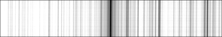
The following excerpt focuses on the H-beta line of neutral hydrogen in the blue region at 4860 angstroms. The line in question is the "deepest" line, located in the center of this image. It's called an absorption line, and it's clear why:

 

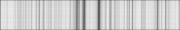
Here is a beautiful region of the solar spectrum, the triplet of the magnesium line (Mg I), which is easily visible at 5170 Ångströms in the green part of the spectrum:

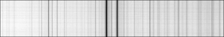
The yellow spectral range is dominated by the famous sodium doublet (Na I). ​​These are the same lines, not absorbing as here, but strongly emitting, that give streetlights in our cities their yellow color (before they were replaced by the cursed LED lamps). We are at a wavelength of approximately 5890 angstroms. Slightly to the left of the sodium lines D1 and D2 (as they are called), in the same spectral range, is the helium line He I at 5873 angstroms (the so-called D3 line). Don't look for this line in the document; it is not visible because it is very weakly emitted compared to the intense continuum (see part 12 of this page):

 

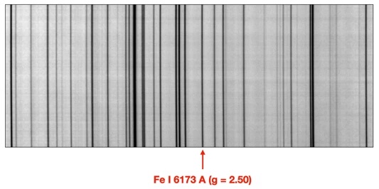
Finally, moving further toward the red, we encounter the H-alpha line of hydrogen, at exactly 6563 angstroms. Note that the spectrum contains fewer and fewer lines from blue to red. This is not an instrumental error, but a very real astrophysical phenomenon. The H-alpha line is thus isolated from its surroundings and easy to detect:

 

In summary, the overall view of the solar spectrum in the visible range looks like this:

 

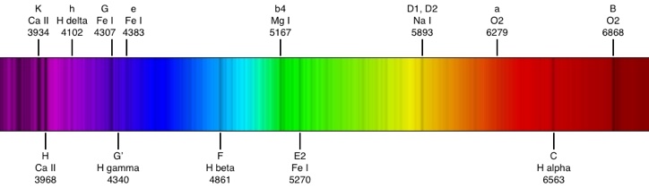
translated from the website: www.astrosurf.com/buil